A step-by-step forward pass and backpropagation example

There are multiple libraries (PyTorch, TensorFlow) that can assist you in implementing almost any neural network architecture. This article is not about solving a neural net using one of those libraries.

Instead, in this article, we'll see a step-by-step forward pass (forward propagation) and backward pass (backpropagation) example. We'll be taking a single hidden layer neural network and solving one complete cycle of forward propagation and backpropagation.

Getting to the point, we will work step by step to understand how weights are updated in neural networks. The way a neural network learns is by updating its weight parameters during the training phase. There are multiple concepts needed to fully understand the working mechanism of neural networks: linear algebra, probability, and calculus. I'll try my best to revisit calculus for the chain rule concept. I will keep aside the linear algebra (vectors, matrices, tensors) for this article. We'll work on each and every computation, and in the end up we'll update all the weights of the example neural network for one complete cycle of forward propagation and backpropagation.

Let's get started.

Here's a simple neural network on which we'll be working.

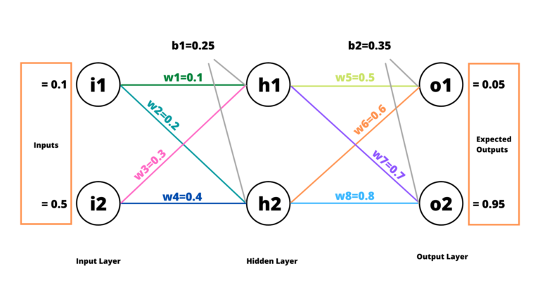
I think the above example neural network is self-explanatory. There are two units in the Input Layer, two units in the Hidden Layer and two units in the Output Layer. The w1, w2, w2, ..., w8 represent the respective weights. b1 and b2 are the biases for Hidden Layer and Output Layer, respectively.

In this article, we'll be passing two inputs i1 and i2, and perform a forward pass to compute the total error and then a backward pass to distribute the error inside the network and update weights accordingly.

Before getting started, let us deal with two basic concepts which should be sufficient to comprehend this article.

Peeking inside a single neuron

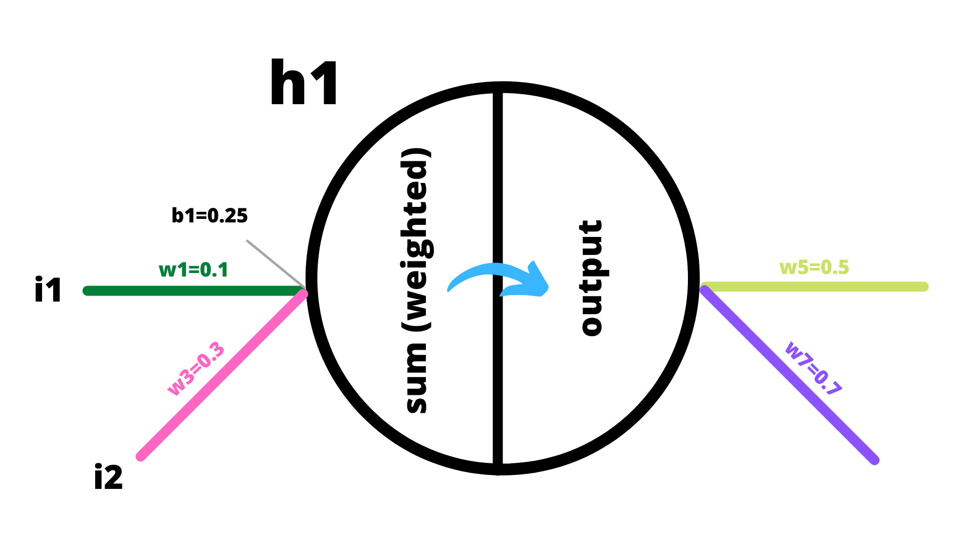
Inside a unit, two operations happen: (i) computation of the weighted sum and (ii) squashing of the weighted sum using an activation function. The result from the activation function becomes an input to the next layer (until the next layer is an Output Layer). In this example, we'll be using the Sigmoid function (Logistic function) as the activation function. The Sigmoid function basically takes an input and squashes the value between 0 and +1.

Chain Rule in Calculus

If we have \(y = f(u)\) and \(u = g(x)\), then we can write the derivative of y as:

\[\frac{dy}{dx} = \frac{dy}{du} * \frac{du}{dx}\]

The Forward Pass

Remember that each unit of a neural network performs two operations: compute weighted sum and process the sum through an activation function. The outcome of the activation function determines if that particular unit should activate or become insignificant.

Let's get started with the forward pass.

For h1,

\[sum_{h1} = i_{1}*w_{1}+i_{2}*w_{3}+b_{1}\]

\[sum_{h1} = 0.1*0.1+0.5*0.3+0.25 = 0.41\]

Now we pass this weighted sum through the logistic function (sigmoid function) so as to squash the weighted sum into the range (0 and +1). The logistic function is an activation function for our example neural network.

\[output_{h1}=\frac{1}{1+e^{-sum_{h1}}}\]

\[output_{h1}=\frac{1}{1+e^{-0.41}} = 0.60108\]

Similarly for h2, we perform the weighted sum operation \(sum_{h2}\) and compute the activation value \(output_{h2}\).

\[sum_{h2} = i_{1}*w_{2}+i_{2}*w_{4}+b_{1} = 0.47\]

\[output_{h2} = \frac{1}{1+e^{-sum_{h2}}} = 0.61538\]

Now, \(output_{h1}\) and \(output_{h2}\) will be considered as inputs to the next layer.

For o1,

\[sum_{o1} = output_{h1}*w_{5}+output_{h2}*w_{6}+b_{2} = 1.01977\]

\[output_{o1}=\frac{1}{1+e^{-sum_{o1}}} = 0.73492\]

Similarly for o2,

\[sum_{o2} = output_{h1}*w_{7}+output_{h2}*w_{8}+b_{2} = 1.26306\]

\[output_{o2}=\frac{1}{1+e^{-sum_{o2}}} = 0.77955\]

Computing the total error

We started off supposing the expected outputs to be 0.05 and 0.95 respectively for \(output_{o1}\) and \(output_{o2}\). Now we will compute the errors based on the outputs received until now and the expected outputs.

We'll use the following error formula,

\[E_{total} = \sum \frac{1}{2}(target-output)^{2}\]

To compute \(E_{total}\), we need to first find out the respective errors at \(o1\) and \(o2\).

\[E_{1} = \frac{1}{2}(target_{1}-output_{o1})^{2}\]

\[E_{1} = \frac{1}{2}(0.05-0.73492)^{2} = 0.23456\]

Similarly, for E2,

\[E_{2} = \frac{1}{2}(target_{2}-output_{o2})^{2}\]

\[E_{2} = \frac{1}{2}(0.95-0.77955)^{2} = 0.01452\]

Therefore, \(E_{total} = E_{1} + E_{2} = 0.24908\)

The Backpropagation

The aim of backpropagation (backward pass) is to distribute the total error back to the network so as to update the weights in order to minimize the cost function (loss). The weights are updated in such as way that when the next forward pass utilizes the updated weights, the total error will be reduced by a certain margin (until the minima is reached).

For weights in the output layer (w5, w6, w7, w8)

For w5,

Let's compute how much contribution w5 has on \(E_{1}\). If we become clear on how w5 is updated, then it would be really easy for us to generalize the same to the rest of the weights. If we look closely at the example neural network, we can see that \(E_{1}\) is affected by \(output_{o1}\), \(output_{o1}\) is affected by \(sum_{o1}\), and \(sum_{o1}\) is affected by \(w5\). It's time to recall the Chain Rule.

\[\frac{\partial E_{total}}{\partial w5} = \frac{\partial E_{total}}{\partial output_{o1}} * \frac{\partial output_{o1}}{\partial sum_{o1}} * \frac{\partial sum_{o1}}{\partial w5}\]

Let's deal with each component of the above chain separately.

Component 1: partial derivative of Error w.r.t. Output

\[E_{total} = \sum \frac{1}{2}(target-output)^{2}\]

\[E_{total} = \frac{1}{2}(target_{1}-output_{o1})^{2} + \frac{1}{2}(target_{2}-output_{o2})^{2}\]

Therefore,

\[\frac{\partial E_{total}}{\partial output_{o1}} = 2*\frac{1}{2}*(target_{1}-output_{o1})*-1\]

\[= output_{o1} - target_{1}\]

Component 2: partial derivative of Output w.r.t. Sum

The output section of a unit of a neural network uses non-linear activation functions. The activation function used in this example is Logistic Function. When we compute the derivative of the Logistic Function, we get:

\[\sigma(x) = \frac{1}{1+e^{-x}}\]

\[\frac{\mathrm{d}}{\mathrm{dx}}\sigma(x) = \sigma(x)(1-\sigma(x))\]

Therefore, the derivative of the Logistic function is equal to output multiplied by (1 - output).

\[\frac{\partial output_{o1}}{\partial sum_{o1}} = output_{o1} (1 - output_{o1})\]

Component 3: partial derivative of Sum w.r.t. Weight

\[sum_{o1} = output_{h1}*w_{5}+output_{h2}*w_{6}+b_{2}\]

Therefore,

\[\frac{\partial sum_{o1}}{\partial w5} = output_{h1}\]

Putting them together,

\[\frac{\partial E_{total}}{\partial w5} = \frac{\partial E_{total}}{\partial output_{o1}} * \frac{\partial output_{o1}}{\partial sum_{o1}} * \frac{\partial sum_{o1}}{\partial w5}\]

\[\frac{\partial E_{total}}{\partial w5} = [output_{o1} - target_{1} ]* [output_{o1} (1 - output_{o1})] * [output_{h1}]\]

\[\frac{\partial E_{total}}{\partial w5} = 0.68492 * 0.19480 * 0.60108\]

\[\frac{\partial E_{total}}{\partial w5} = 0.08020\]

The \(new\_w_{5}\) is,

\(new\_w_{5} = w5 - n * \frac{\partial E_{total}}{\partial w5}\), where n is learning rate.

\[new\_w_{5} = 0.5 - 0.6 * 0.08020\]

\[new\_w_{5} = 0.45187\]

We can proceed similarly for w6, w7 and w8.

For w6,

\[\frac{\partial E_{total}}{\partial w6} = \frac{\partial E_{total}}{\partial output_{o1}} * \frac{\partial output_{o1}}{\partial sum_{o1}} * \frac{\partial sum_{o1}}{\partial w6}\]

The first two components of this chain have already been calculated. The last component \(\frac{\partial sum_{o1}}{\partial w6} = output_{h2}\).

\[\frac{\partial E_{total}}{\partial w6} = 0.68492 * 0.19480 * 0.61538 = 0.08211\]

The \(new\_w_{6}\) is,

\[new\_w_{6}= w6 - n * \frac{\partial E_{total}}{\partial w6}\]

\[new\_w_{6} = 0.6 - 0.6 * 0.08211\]

\[new\_w_{6} = 0.55073\]

For w7,

\[\frac{\partial E_{total}}{\partial w7} = \frac{\partial E_{total}}{\partial output_{o2}} * \frac{\partial output_{o2}}{\partial sum_{o2}} * \frac{\partial sum_{o2}}{\partial w7}\]

For the first component of the above chain, let's recall how the partial derivative of Error is computed w.r.t. Output.

\[\frac{\partial E_{total}}{\partial output_{o2}} = output_{o2} - target_{2}\]

For the second component,

\[\frac{\partial output_{o2}}{\partial sum_{o2}} = output_{o2} (1 - output_{o2})\]

For the third component,

\[\frac{\partial sum_{o2}}{\partial w7} = output_{h1}\]

Putting them together,

\[\frac{\partial E_{total}}{\partial w7} = [output_{o2} - target_{2}] * [output_{o2} (1 - output_{o2})] * [output_{h1}]\]

\[\frac{\partial E_{total}}{\partial w7} = -0.17044 * 0.17184 * 0.60108\]

\[\frac{\partial E_{total}}{\partial w7} = -0.01760\]

The \(new\_w_{7}\) is,

\[new\_w_{7} = w7 - n * \frac{\partial E_{total}}{\partial w7}\]

\[new\_w_{7} = 0.7 - 0.6 * -0.01760\]

\[new\_w_{7} = 0.71056\]

Proceeding similarly, we get \(new\_w_{8} = 0.81081\) (with \(\frac{\partial E_{total}}{\partial w8} = -0.01802\)).

For weights in the hidden layer (w1, w2, w3, w4)

Similar calculations are made to update the weights in the hidden layer. However, this time the chain becomes a bit longer. It does not matter how deep the neural network goes; all we need to find out is how much error is propagated (contributed) by a particular weight to the total error of the network. For that purpose, we need to find the partial derivative of Error w.r.t. to the particular weight. Let's work on updating w1, and we'll be able to generalize similar calculations to update the rest of the weights.

For w1 (with respect to E1),

For simplicity let us compute \(\frac{\partial E_{1}}{\partial w1}\) and \(\frac{\partial E_{2}}{\partial w1}\) separately, and later we can add them to compute \(\frac{\partial E_{total}}{\partial w1}\).

\[\frac{\partial E_{1}}{\partial w1} = \frac{\partial E_{1}}{\partial output_{o1}} * \frac{\partial output_{o1}}{\partial sum_{o1}} * \frac{\partial sum_{o1}}{\partial output_{h1}} * \frac{\partial output_{h1}}{\partial sum_{h1}} * \frac{\partial sum_{h1}}{\partial w1}\]

Let's quickly go through the above chain. We know that \(E_{1}\) is affected by \(output_{o1}\), \(output_{o1}\) is affected by \(sum_{o1}\), \(sum_{o1}\) is affected by \(output_{h1}\), \(output_{h1}\) is affected by \(sum_{h1}\), and finally \(sum_{h1}\) is affected by \(w1\). It is quite easy to comprehend, isn't it?

For the first component of the above chain,

\[\frac{\partial E_{1}}{\partial output_{o1}} = output_{o1} - target_{1}\]

We've already computed the second component. This is one of the benefits of using the chain rule. As we go deep into the network, the previous computations are reusable.

For the third component,

\[sum_{o1} = output_{h1}*w_{5}+output_{h2}*w_{6}+b_{2}\]

\[\frac{\partial sum_{o1}}{\partial output_{h1}} = w5\]

For the fourth component,

\[\frac{\partial output_{h1}}{\partial sum_{h1}} = output_{h1}*(1-output_{h1})\]

For the fifth component,

\[sum_{h1} = i_{1}*w_{1}+i_{2}*w_{3}+b_{1}\]

\[\frac{\partial sum_{h1}}{\partial w1} = i_{1}\]

Putting them all together,

\[\frac{\partial E_{1}}{\partial w1} = \frac{\partial E_{1}}{\partial output_{o1}} * \frac{\partial output_{o1}}{\partial sum_{o1}} * \frac{\partial sum_{o1}}{\partial output_{h1}} * \frac{\partial output_{h1}}{\partial sum_{h1}} * \frac{\partial sum_{h1}}{\partial w1}\]

\[\frac{\partial E_{1}}{\partial w1} = 0.68492 * 0.19480 * 0.5 * 0.23978 * 0.1 = 0.00159\]

Similarly, for w1 (with respect to E2),

\[\frac{\partial E_{2}}{\partial w1} = \frac{\partial E_{2}}{\partial output_{o2}} * \frac{\partial output_{o2}}{\partial sum_{o2}} * \frac{\partial sum_{o2}}{\partial output_{h1}} * \frac{\partial output_{h1}}{\partial sum_{h1}} * \frac{\partial sum_{h1}}{\partial w1}\]

For the first component of the above chain,

\[\frac{\partial E_{2}}{\partial output_{o2}} = output_{o2} - target_{2}\]

The second component is already computed.

For the third component,

\[sum_{o2} = output_{h1}*w_{7}+output_{h2}*w_{8}+b_{2}\]

\[\frac{\partial sum_{o2}}{\partial output_{h1}} = w7\]

The fourth and fifth components have also already been computed while computing \(\frac{\partial E_{1}}{\partial w1}\).

Putting them all together,

\[\frac{\partial E_{2}}{\partial w1} = \frac{\partial E_{2}}{\partial output_{o2}} * \frac{\partial output_{o2}}{\partial sum_{o2}} * \frac{\partial sum_{o2}}{\partial output_{h1}} * \frac{\partial output_{h1}}{\partial sum_{h1}} * \frac{\partial sum_{h1}}{\partial w1}\]

\[\frac{\partial E_{2}}{\partial w1} = -0.17044 * 0.17184 * 0.7 * 0.23978 * 0.1 = -0.00049\]

Now we can compute \(\frac{\partial E_{total}}{\partial w1} = \frac{\partial E_{1}}{\partial w1} + \frac{\partial E_{2}}{\partial w1}\).

\(\frac{\partial E_{total}}{\partial w1} = 0.00159 + (-0.00049) = 0.00110\).

The \(new\_w_{1}\) is,

\[new\_w_{1} = w1 - n * \frac{\partial E_{total}}{\partial w1}\]

\[new\_w_{1}= 0.1 - 0.6 * 0.00110\]

\[new\_w_{1} = 0.09933\]

Proceeding similarly, we can easily update the other weights (w2, w3 and w4).

\[new\_w_{2} = 0.19919\]

\[new\_w_{3} = 0.29667\]

\[new\_w_{4} = 0.39597\]

Once we've computed all the new weights, we need to update all the old weights with these new weights. Once the weights are updated, one backpropagation cycle is finished. Now the forward pass is done and the total new error is computed. And based on this newly computed total error the weights are again updated. This goes on until the loss value converges to minima. This way a neural network starts with random values for its weights and finally converges to optimum values.

I hope you found this article useful. I'll see you in the next one.